

Abstract
Pressure Transient Analysis (PTA) provides valuable information about the subsurface completion and reservoir. Permanent downhole pressure gauges (PDHG) are not always available in wells. In such cases, wellhead pressure (WHPG) gauges or temporary downhole gauges (DHG) can be used to perform reservoir/ completion diagnostics. Although in some cases, it is safe to use raw WHP data for analysis, in a lot of cases, it should not be done. Fair et al. (2002) presented a methodology to categorize wells that could be tested from the surface (well head) along with a methodology that allows surface-to-bottomhole pressure (BHP) conversion.
A few authors in the past have emphasized the importance of converting wellhead pressure and downhole gauge pressure data to mid-completion bottomhole conditions to account for friction and changing fluid density during a test. Performing PTA without correcting the gauge data for these wellbore effects can lead to inaccurate results: especially the over-estimation of skin and permeability, and underestimation of P*, and in-place hydrocarbon volumes, due to reservoir signal suppression. The WHP data could also be nonanalyzable (using conventional methods) if the effects are severe. Hakim et al. (2016) further discussed the importance of this conversion and presented examples where WHP to BHP conversions in various types of wells could be performed with high accuracy using a coupled PVT-thermal wellbore model.
This paper will introduce the concept of rate of change in wellbore fluid density (wellbore signal) relative to the rate of reservoir pressure increase/decrease (reservoir signal) during a test. The purpose is to identify the factors affecting the “reservoir signal” in the measured wellhead pressure and rate data during a well flowback and during the commercial production period and to provide guidelines to help the petroleum engineer determine the severity of these factors in a given well/reservoir system. This should help the petroleum engineer in deciding whether to rely on the WHP data or run a DHG to observe the reservoir signal.
A 3-step methodology to determine the magnitude of the wellbore signal relative to the reservoir signal will be presented with solved examples of an oil well and a gas-condensate well.
Introduction
The reservoir signal is the pressure response of the reservoir at the sand face, commonly referred to as ‘true bottomhole pressure’ or ‘datum pressure’, or just BHP. During a buildup test (PBU) the BHP generally increases and during a drawdown test (DD) the BHP generally decreases. The nature of the change in pressure is indicative of the various reservoir flow regimes a well is experiencing such as wellbore storage, radial flow, pseudo steady-state flow, linear flow, etc. Reservoir characteristics such as transmissibility, permeability-thickness (flow capacity), permeability, skin, reservoir limits, etc. are obtained via analysis of the reservoir signal.
A pressure gauge measures the reservoir signal through a column of fluid in the well bore that is in hydraulic communication with the reservoir, below the gauge. This column of fluid could be thousands of feet in height and is subject to frictional pressure losses (if the well is flowing), and density variations caused by changing temperature and pressure, especially for compressible fluids. This introduces a wellbore signal to the measured data, masking (usually suppressing) the reservoir signal partially, or completely. In short, a pressure gauge measures a pressure that is a function of changing fluid properties and flowing conditions below the gauge AND the reservoir signal. It is important to mention that testing a well from the surface is only possible if the well is not loading (efficiently lifting produced liquid) and that this paper does not address the problems associated with phase re-segregation in a PBU. If phase re-segregation is a likely issue, the authors recommend performing a 2-rate test to evaluate completion/reservoir parameters.
Defining the Reservoir Signal
The reservoir signal is the rate of change of pressure per unit time. On a Cartesian scale, it has the units of psi/sec, psi/min, psi/hr or psi/day and so on. On a Semi-log scale, the radial flow slope, m (psi/cycle), is a straight-line (time is measured in hours). If the well is no longer undergoing infinite acting radial flow, the slope deviates from straight-line behavior towards another straight-line with a different slope (for ex: when encountering any reservoir boundaries) or towards curvature (linear flow in a channel or pseudo-steady state flow). The reservoir signal, as measured at the mid-completion depth, is the true reservoir signal. The higher up the measurement point along the wellbore, the weaker the reservoir signal becomes due to the addition of the wellbore signal. This is discussed in detail in the next section.

Defining the Wellbore Signal
It is important to remember the following fundamental relationship between WHP and BHP (ignoring friction for simplicity):

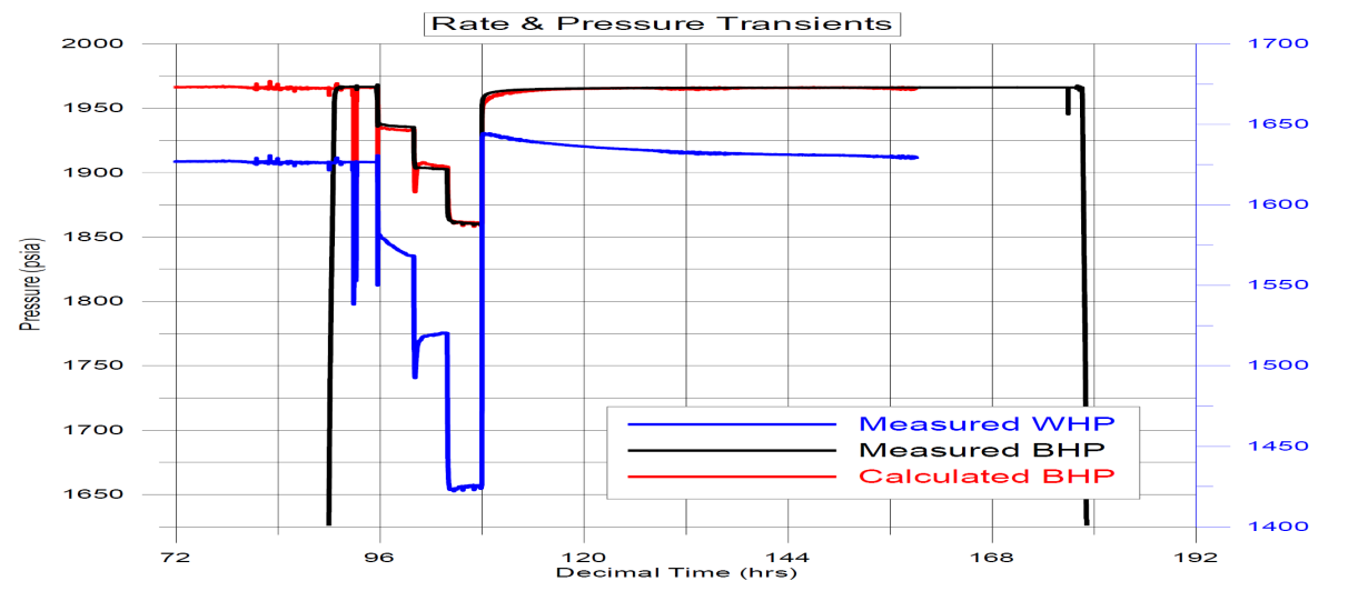
Figure 1 - WHP Increase in a DD/Decrease in a PBU
Life would be much simpler (and much more boring for the authors) if the change in WHP mirrored the change in BHP. Unfortunately, this is rarely the case in wells with a small reservoir signal because of changing fluid density in the wellbore, such as the well in Fig.1. The reservoir signal is the ΔBHP term and the wellbore signal is the Δρgh term. In a shut-in, the ΔBHP term increases due to increasing bottomhole pressure and the Δρgh term also increases because of the increase in fluid density due to wellbore cooling and due to increased pressure. In a drawdown, the opposite happens and the Δρgh term decreases. If the wellbore signal changes more rapidly (due to density changes) as compared to the reservoir signal, the reservoir signal will be masked (partially or completely) and the ΔWHP term is suppressed.
High permeability wells are more susceptible to wellbore signal masking the reservoir signal as compared to low permeability wells. High permeability wells have a lower mid-time slope/reservoir signal (m, psi/ cycle) and the rate of bottomhole pressure increase/decrease (ΔBHP) is smaller. Low permeability wells have a higher mid-time slope (m, psi/cycle) and the rate of BHP increase/decrease is greater. It can be said that the reservoir signal is relatively smaller in higher permeability wells as compared to their low permeability counterparts.
The severity of the wellbore signal is dependent on the following key parameters:
1. Fluid compressibility: The more compressible the fluid, the greater the density variation with pressure and temperature, the greater the wellbore signal. This means that gas and gas-condensate wells are especially susceptible to masking/suppression of the reservoir signal.
2. Deviation of dynamic (flowing) wellbore thermal gradient from static (shut-in) gradient: After a well is shut-in, the fluid molecules at any given depth approach equilibrium with the earth’s temperature at that depth (aka geothermal gradient). However, during flowing conditions, the warmer reservoir fluid travels up the well bore, losing heat to the surroundings. The temperature at any given point along the tubing then depends on the fluid velocity, the heat capacity of the fluid, the heat lost to the surroundings, and the time/production history. During a PBU or DD, a thermal transient is initiated and the temperature profile shifts from the static equilibrium temperature profile to the new flowing temperature profile and vice versa. The greater the deviation in these profiles, the greater the ΔT the fluid is exposed to, the greater the density change, and the greater the wellbore signal.
3. Reservoir transmissibility (kh/μ): The higher the formation transmissibility, the smaller the reservoir signal compared to the wellbore signal (for a given fluid). The formation transmissibility can be estimated to predict whether the well falls under the danger zone (wellbore signal significantly affecting the reservoir signal) prior to the flowback/well test.

Transmissibility can be classified in the following ranges (in order of decreasing reservoir signal strength): If an oil or gas well falls under the low transmissibility range, the reservoir signal will be strong compared to the wellbore signal (density change due to temperature changes) and the data is not susceptible to getting masked by the wellbore signal. Moderate transmissibility oil wells have a small wellbore signal but moderate transmissibility gas wells are susceptible to the wellbore signal masking the reservoir signal just enough to cause slope suppression and impact PTA and reservoir analyses. In moderately-high transmissibility oil wells, the data could possibly be severely affected by the wellbore signal but analysis might still be possible. In moderately-high transmissibility gas wells, it is not recommended to rely on raw WHP data at all (in some cases raw data might be non-analyzable). Oil wells, in general, can handle a smaller reservoir signal (larger kh/μ) due to smaller density variation in the wellbore compared to gas wells. In high transmissibility wells, a permanent DHG should be installed or a rigorous WHP to BHP conversion should be performed using a coupled PVT-thermal wellbore model.
Please note that this applies only to single phase wells. For multi-phase wells, see the discussion below.
4. Number of fluid phases present in the wellbore (especially during a PBU): If there’s more than one fluid phase present in the wellbore at the time of shut-in, gravity segregation will occur once there isn’t enough velocity to lift/mix the fluids. The greater the difference in fluid properties of these phases, the stronger the wellbore signal, and the more masked the WHP response will be. Even with a DHG present, things get very complicated if there is a moving fluid interface below the DHG (re-injection into the formation). If the well meets the criteria for a small impact wellbore signal, these types of wells may be tested by performing a 2-rate test (Example: If the well is lifting efficiently at 1,000 BOPD with free gas and water, reduce the choke to target 600 BOPD or some lesser rate that is still lifting efficiently, then return to the previous choke).
5. Distance from mid-perforation depth: The further away the pressure measurement location from the mid-perforation depth, the larger the wellbore signal. In other words, as the distance from the mid-perforation depth increases along the wellbore, the temperature change (and consequent density change) increases, and the wellbore signal increases. This causes the observed ‘reservoir signal’ to be masked/suppressed. The highest wellbore signal (upstream of the choke) is at the wellhead pressure gauge. However, a DHG at significant heights above the completion is also susceptible to the same wellbore effects as the surface gauge. For this reason, even DHG data should always be corrected to mid-perforation depth for vertical wells and to the top of the completion for horizontal/deviated wells.
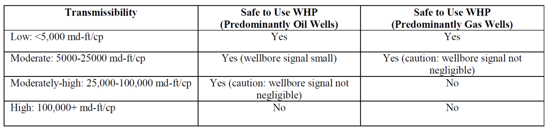
Table 1 - Characterization of Wells by Reservoir Transmissibility
These topics have been covered in greater detail by Hakim et. al (2016). It can be concluded that (aside from fluid re-segregation) the wellbore signal is dominated by the extent of temperature change the fluid is exposed to, the extent of density changes the fluid experiences due to the temperature change and the number of phases present. The objective of this paper is to allow the reader to determine whether the reservoir signal in a particular well is expected to be dominated by the wellbore signal and whether a downhole gauge should be run to overcome this problem.
Flowbacks and Post Clean-Up Well Production
This section has been divided into two subsections: flowbacks and post clean-up well production. The objective is to breakdown the factors affecting the captured pressure and rate data, and reservoir analysis during each of these periods.
Reservoir transmissibility
The reservoir permeability, k (md), can be estimated based on nearby wells or other analogs. The estimate needs to be close (same order of magnitude as the actual permeability) but not perfect. Often much better estimates of the permeability are obtained from the first few PBU or DD tests during a flowback. The net TST pay, h, can be estimated from the well logs with reasonably good certainty (as long as the well deviation and the dip of the formation are considered). The viscosity can easily be estimated using correlations or an EOS (Equation of State) from a nearby well/analog fluid, and surface or downhole fluid sample PVT analysis. Once the transmissibility (kh/μ [=] md-ft/cp) is estimated, a decision to run DHGs can be made prior to the flowback. It is recommended to also use this method to make a decision about installing permanent DHGs during the well/completion design, to capture and analyze long-term production data.
Pressure measurement
As a minimum, a well should be equipped with a surface pressure gauge during flowback operations. It would be extremely beneficial to have a DHG present in the well during the flowback but it’s not always feasible. Modern pressure gauges are far superior in quality and more cost-friendly compared to their predecessors from a few decades ago and have high gauge resolution in both temperature and pressure. Moreover, data frequency and storage are no longer considered a big issue. Without pressure data, one would be “flying blind”. For example, a well could be undergoing liquid loading, or productivity damage due to excessive drawdown. Without monitoring pressure data, it would be really hard to identify these effects. Measuring and recording flowback data also provides an early “quick look” opportunity into the completion and formation characteristics; normally such information is obtained much later in the life of a well, i.e. after the well has cleaned-up and brought back online for commercial production.
Rate measurement
Flowrate is an extensive, inferred property. There is no such thing as a direct flowrate measurement. Flowrate calculations are performed by measuring another property such as pressure drop or volume and time. The importance of accurate flow rates (in addition to pressure measurement) cannot be emphasized enough. Accurate pressure measurement coupled with flowrate measurement can enable flowback optimization, that could result in a successful flowback, a properly cleaned-up well, better choke management, more accurate PTA reserves estimates, etc. For gas rate measurement via orifice plate or venturi flowmeters, it is recommended to stay within 20-80% of the scale for accurate flowrate calculation and ensure all the right input parameters are entered into the calculation engine/program. For example, a Daniels Orifice Flow Calculator requires inputs such as operating pressure and temperature, pipe size, density, specific gravity, differential pressure, orifice bore diameter, beta ratio, etc. For oil wells, one should ensure that any rate ‘measurement’ equipment/device is calibrated properly. For test separator rates, it is recommended that for a given choke setting, the rate should be a weighted average over a reasonable time (a few hours) instead of relying on individual measurements.
Flowbacks
Every well goes through a flowback in the early stages of its life. A flowback refers to producing back the well’s completion fluid (and/or frac fluid) to enable hydrocarbon production from the reservoir. Flowbacks were once considered a necessary evil and unimportant from a data capture and analysis standpoint. However, flowbacks are now getting the attention they deserve and the trend has shifted towards capturing and analyzing flowbacks. After all, a flowback is nothing but a very complicated well test problem that can yield valuable information very early in the life of the well, enabling better decision-making. Flowbacks can be subdivided into 2 main categories:
1. Conventional flowbacks: In a conventional flowback, the completion fluid is followed by
hydrocarbons.
2. Frac flowbacks: In a frac flowback, the well is usually filled with flush fluid from the frac job. During the flowback, the flush fluid is produced, followed by the frac fluid from the various stages prior to the flush. Frac flowbacks are complicated in the sense that it is really difficult to exactly know what’s in the wellbore at a given time.
Displacement
Sometime after the flowback has begun, hydrocarbon production commences. Generally, the hydrocarbon production increases gradually while the completion/frac fluid production decreases (more of a swap in the fraction of completion fluid in the wellbore). This process is known as displacement. The head in the wellbore continuously decreases due to production of the lighter hydrocarbon fluids (unless it’s heavy, dead oil). This results in a very strong wellbore signal and causes the WHP or (apparent converted BHP) to rise. This is nothing to worry about. After the density inversion is over, the WHP should start resembling a reservoir response.
Wellbore Warming
As a well is brought online for a flowback, the wellbore undergoes warming. The cooler fluid is being replaced by warmer fluid from the reservoir. This effect lowers the wellbore fluid density and results in an increase in WHP (although the response will initially be dominated by density inversion).
Skin reduction
During a flowback (and post-flowback production), some of the debris and mud filtrate is also recovered, resulting in a gradual skin improvement with continued production. This causes the flowing pressure to increase due to a lower ΔPskin. Monitoring PBU/DD skin values can confirm this.
Increasing Gas Liquid Ratio (GLR)
The producing GLR can increase rather rapidly in a short period of time. This could be due to a few reasons such as – density inversion in a gas well, increased contribution to flow from a gas cap/zone being commingled with oil, changing reservoir composition due to pressure depletion etc. Whatever may be the reason, this results in a decreasing wellbore density and increasing WHP. This can be confirmed by looking for a gas rate increase from the separator.
Liquid (water) loading
If the hydrocarbon rate is not sufficient to lift all the fluids from the bottom of the well efficiently (full sweep), then the well is considered to be partially or fully loading. A column of heavy fluid forms at the bottom of the wellbore and the surface pressure drops quickly.
Reservoir response
Once most of the completion fluid/frac fluid is recovered, skin clean-up has been completed and produced fluid property variation has stopped occurring, the (WH) pressure response may start to resemble a reservoir response. At this point, it is crucial to take fluid samples for field evaluation (API gravity, viscosity measurement etc.) or a detailed lab analysis to understand the produced fluid and set a benchmark. This fluid property information can then be used for BHP conversion and also creating/tuning an EOS for reservoir analysis.
Post Clean-up Well Production
In this phase, some of the wellbore effects that were dominant during the flowback phase are no longer dominant, although those effects may still be present or may present themselves later in the life of the well. In general, skin reduction may continue to occur even in this phase but usually stops occurring in a few days/weeks. Displacement (which was one of the most dominant effects in the flowback phase) should no longer be dominant provided that the well has produced most of the completion and/or frac fluid back and is now producing mostly hydrocarbons. Wellbore warming effects will still be present in gas, gas-condensate and volatile oil wells, masking the response during every new transient/rate change. Liquid loading could occur if the flow rates are low (below the critical lifting rate). Liquid fallback and re-injection may still be a problem in multi-phase gas or oil wells during shut-in conditions, often masking the radial flow reservoir response during early-time. Increasing GLR during the production phase will also introduce a wellbore signal – this could occur below bubble point or if contribution from the gas cap increases. Similar effects can be seen in gas-condensate wells with condensate drop-out. During stabilized production, if a straight-line response on a pressure vs time plot is present (indicative of PSS or SS flow regime) at relatively constant rates, then the reservoir response is likely valid. If it is difficult to achieve this, a DHG should be run.
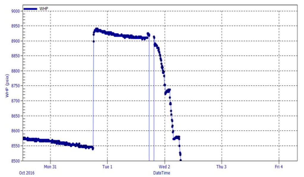
Flowback example
The following example is of a fracture-stimulated oil well that had been partially unloaded of frac fluid and shut-in. Fortunately, there was a DHG present in the well during this flowback. The downhole gauge is more representative of the reservoir response at all times and the difference in the DHGP and the WHP can be used to calculate the wellbore gradient (psi/ft). Th wellbore gradient calculation helps differentiate between reservoir and wellbore effects. The DHGP and the wellbore gradient (psi/ft) will be used for explanation purposes since it is available but the WHP by itself can be sufficient to help identify many events.
Figure 2 - Fracture-Stimulated Oil Well Flowback
1. Shut-in. The well is initially shut-in.
2. Flowback begins. The well initially produces lighter fluid at the surface. The WHP (blue) decreases, the DHGP (orange) decreases and the flowing gradient (purple) decreases slightly. The increase in the wellbore gradient is caused by friction.
3. Producing Frac Fluid. Heavier fluid (frac fluid) enters the wellbore. The WHP decreases rapidly, the DHGP keeps decreasing (reservoir response dominated), the flowing gradient increases rapidly.
4. Displacement. The frac fluid is followed by lighter fluid (oil). Over the next few hours, the WHP increases, the DHGP continues to decrease, the flowing wellbore gradient decreases rapidly. Towards the end of this stage the flowing gradient stabilizes, but the well is still making some completion/frac fluid (still ‘cleaning up’).
5. Additional Oil. As the drawdown increases, additional oil volume is produced. The WHP now starts to decrease, DHGP continues to decrease, the flowing wellbore gradient decreases rapidly.
6. Additional frac fluid. Due to the increased drawdown, additional frac fluid from within the reservoir and wellbore is produced. The well is said to be “belching” heavy frac fluid. This is similar to stage 3.
7. Shut-in. The well is shut-in to perform pressure transient analysis and get a “feel” for the skin, PI, permeability and near well boundaries. The fluid in the well bore ‘layer-cakes’, with the light fluid rising to the top and heavier fluids falling to the bottom of the well.
8. Flowback continues. The well briefly produces additional frac fluid after coming back online, indicated by the steeply declining WHP and the increasing wellbore gradient. In about 3 hours, the WHP ceases decreasing as rapidly (even increases a bit) and the flowing gradient decreases, indicating production of lighter fluid (oil). After this surge of frac/completion fluid is over, the well produces mostly oil. The WHP response starts to somewhat mimic the DHGP response.
9. Reservoir response dominates? The WHP response mimics the DHGP response and starts to look like a reservoir response (smoothly decaying pressure at a fixed choke). Where the WHP seems to mimic the DHGP and reservoir response, the WHP indicates a slope of 545 psi/d but the DHGP indicates a slope of 661 psi/d; a difference of approximately 20%. This proves that even when it appears that wellbore effects are absent, the reservoir signal may be affected by wellbore signals.
Note: Skin clean-up is an ongoing effect and can be verified between one PBU/DD test to another. If the flowrate measurement is accurate and continuous, skin clean-up can be identified when the flowing pressures increase slightly/or decrease less while the rate increases. In this example, the rate measurement was not as frequent and there was no individual event that stood out as skin clean-up during the flow. However, between consecutive PBU analyses, there was some improvement in the skin.
Discussion/Things to Note
1. The WHP data can be converted to BHP if the flowrates are measured accurately and accurate fluid properties are available. However, the raw WHP data should NOT be trusted as-is. Alternatively, DHPG data can be used for analysis if there is a DHG present close to the mid-completion depth (with scalar correction for the depth offset).
2. It is important to recognize the various wellbore effects in order to not confuse the observations with a reservoir response.
3. Even if wellbore effects seem to be absent and the reservoir response seems to prevail, the wellbore signals may be masking the reservoir signal. The engineer should be extremely careful before making the decision to trust the WHP data. If the WHP does not seem trustworthy, a DHG should be installed.
Estimating Effect of Wellbore Signal on the Reservoir Signal
The various factors affecting the reservoir signal have been covered in the previous sections. How can an engineer quickly determine the extent of the wellbore signal relative to the reservoir signal for a particular well? A simple exercise demonstrated below can guide the engineer in the right direction regarding running a DHG in the well.

Assuming the density of the fluid at the completion doesn’t vary significantly, the above equation can be simplified:

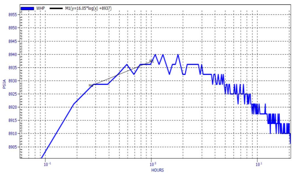
The difference in density of the fluid at the surface at 1 hr and 0.1 hr represents the density change in 1 log cycle. This value will then be compared with the reservoir signal during the same log cycle. For practical simplicity, instead of the density at 0.1 hr, the density at ISIP (instantaneous shut-in pressure) conditions can be used.
If the well is a moderately-high or a high transmissibility gas or oil well, it will be susceptible to a small reservoir signal and a possibly a high wellbore signal. Steps 2 and 3 can confirm this by comparing the reservoir signal to the expected wellbore signal. If the wellbore signal is similar or greater in magnitude than the reservoir signal, the WHP data cannot be trusted and a DHG should be run for capturing and analyzing data. A dynamic PVT-thermal model can also be used to correct the data for the density effects in the wellbore.
Single Phase Oil Well Example
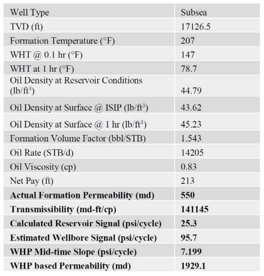
The first step is to determine the transmissibility of this well to categorize this into one of the categories mentioned in Table 1.
1. Calculating the transmissibility

The transmissibility was estimated at 141,145 md-ft/cp. Based on Table 1, this well can be categorized as a high transmissibility well. Just by analyzing the transmissibility, it can be deduced that this well can be expected to have a small reservoir signal.
2. Calculating the reservoir signal (The reservoir signal can be calculated using Eqn.1.)

With a slope of 25 psi/cycle, the reservoir pressure in the well is expected to buildup 25 psi over the next log cycle. This procedure just estimates the reservoir signal (psi/cycle) without the influence of the wellbore signal. In this case (PBU), it is the rate of reservoir pressure increase. The same calculation can be done for a drawdown if needed.
3. Calculating the wellbore signal
In most cases, the majority of the wellbore temperature drop occurs in the first 10 hours. The wellbore temperature drop results in a density increase, which causes the reservoir signal to be suppressed. The temperature drop is minimum at the mid-completion depth and maximum at the wellhead. The increase in pressure in the well bore (wellbore signal) caused by the density increase can be estimated as follows:

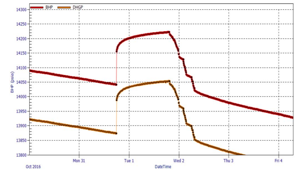
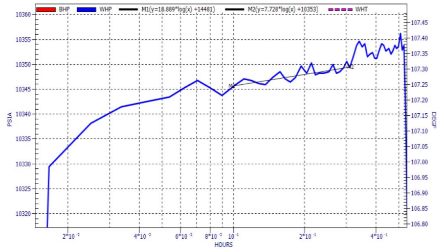
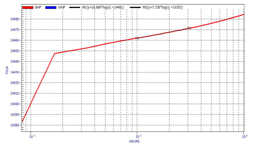
Although the calculated wellbore signal is a very rough estimate, the relative magnitude is enough to indicate that the wellbore signal is strong and will dominate the reservoir signal (95.68 psi over one log cycle compared to 25.25 psi). In Fig.3, the WHP increase is clearly suppressed and eventually completely dominated by the wellbore signal. Any PTA analysis on the raw WHP data would give erroneous results. The permeability estimate from the WHP radial flow period was 1,929 md (actual permeability is close to 550 md), which is a gross overestimation.


2. Calculating the reservoir signal

3. Calculating the wellbore signal

Since the transmissibility is 77,000 md-ft/cp (moderately-high), the reservoir signal can be expected to be relatively small and the WHP should not be trusted as per Table 1. The reservoir signal is estimated at 19 psi/cycle and the wellbore signal is estimated at 21 psi/cycle. The estimated wellbore signal is very similar in magnitude to the reservoir signal. This is also another strong indication that the measured WHP is highly susceptible to being masked by wellbore cooling effects. The PBU was short enough such that the WHP did not start to decrease during the shut-in. This could be very misleading since the effect of the wellbore signal is very subtle in this case and not obvious. The estimated permeability using the WHP mid-time slope is 113 md, more than double the actual formation permeability (46 md).

Gauge Location Effects
Hakim et al. (2016) demonstrated in their 2016 paper how the pressure build-up analysis results varied when the analysis was performed using gauge pressures located at different depths in the well bore and then with the BHP in a high transmissibility gas well. Fig. 11 shows the Semi-log pressure build-up plots and the corresponding mid-time slopes.
Figure 11 - Semi-log plot of WHP, U-DHGP, L-DHGP and BHP
The table below summarizes the Semi-log analysis results:
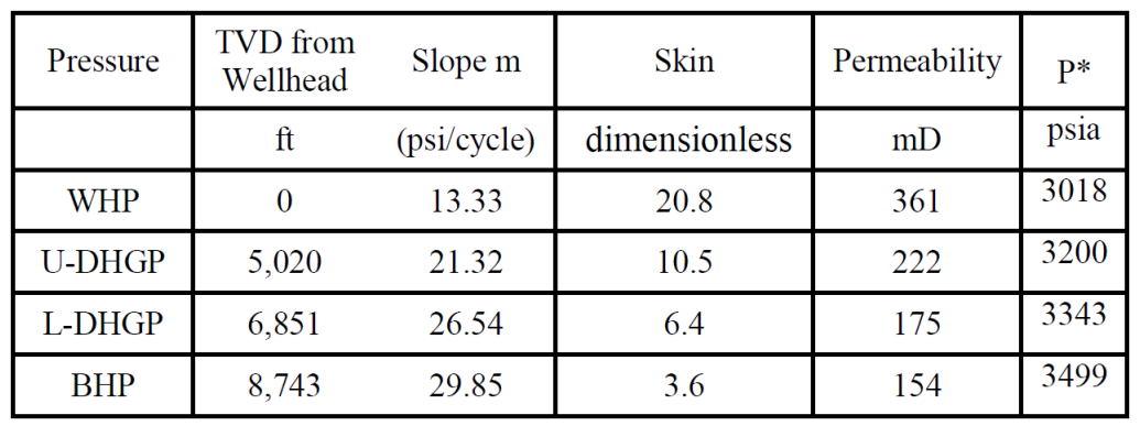
Table 2 - PTA Results
It can be observed (Table 2) that the further the gauge is from the perforations, the smaller the reservoir signal, m (psi/cycle), appears to be (due to the masking effect of the wellbore signal). The calculated permeability and skin increase and the estimated P* decreased the further away the gauge is from the perforations. The 3-step technique mentioned in this paper (calculate transmissibility, reservoir signal, and wellbore signal) can be applied to this well and one would arrive at the conclusion that this well is very susceptible to a high wellbore signal compared to a small reservoir signal.
Conclusions
Gauge data is subject to frictional pressure losses (if the well is flowing), and density variations caused by changing temperature and pressure, especially for compressible fluids, and thus introducing a wellbore signal. A plethora of research, modeling and analysis work has been done using just WHP data without considering the possible implications wellbore effects may have on the measured pressure/temperature data and the results, leading to inaccuracy.
The purpose of this paper is to provide guidelines to the engineer to quickly determine whether a particular well is subject to a high wellbore signal that could be masking/suppressing the reservoir signal. The types of wells and their susceptibility to reservoir signal suppression are characterized based on the reservoir transmissibility (Table 1). A framework to quickly compare the reservoir signal to the wellbore signal to confirm whether a well is likely to have reservoir signal suppression has also been provided.
The factors contributing to the wellbore signal suppression of the reservoir signal are:
-
-
- Fluid compressibility
- Deviation of dynamic (flowing) wellbore thermal gradient from the static (shut-in) gradient
- Formation transmissibility (kh/μ)
- Number of fluid phases present in the wellbore (especially during a PBU)
- Distance from the mid-perforation depth (TOC for a horizontal well)
-
A few situations that can lead to a high wellbore signal in the life of a well are also pointed out:
-
-
- Displacement
- Wellbore Warming (drawdowns or rate increases) and Cooling (PBUs and rate reductions)
- Skin reduction
- Changing Gas-Liquid Ratios
- Liquid (water) loading
-
If an engineer uses the guidelines mentioned in this paper to determine the extent of the wellbore signal relative to the reservoir signal, he/she should be able to quickly determine if a well needs to have a downhole gauge (run close to the completion depth), or if uncorrected WHPs will suffice. This determination can also be performed as part of the well/completion design in order to determine if the well needs to be kitted up with a downhole permanent gauge.
The reader should also be aware that there are methods available to account for wellbore physics, employing a rigorous PVT-thermal wellbore model to convert raw WHP data to mid-completion BHP before performing any analysis. However, if this technology is not available, it may be best to just run a DHG anyway.
Acknowledgements
The authors would like to thank Don Nguyen, Hardy Soni, and Lidia E Pinzon R for their time and effort in reviewing this paper.