

See the presentation associated with this technical paper here: https://www.odsi-energy.com/ODSI-inertia-derivation-diffusion-equation-presentation
See the video associated with this technical paper here: https://www.odsi-energy.com/ODSI-inertia-derivation-diffusion-equation-video
Abstract
When flow is initiated from a well, a physical shock front is created in the reservoir, beginning at the completion. This shock front moves out into the reservoir as a Mechanical Wave with constant intensity and with velocity decreasing vs. the square of the distance. This is known as infinite acting radial flow (aka ‘transient flow’) and is very well understood (at least at the producing well’s location). The capillary shockwave represents a moving boundary to the pressure decay field that forms around the well (Hurst 1934). This active region of decay behind the moving shock front will adopt a near semisteady state flow regime in the reservoir, as required by the second law of thermodynamics. This depletion region is composed of radial capillaries that produce flow to the well and create pressure or elastic depletion in the reservoir. The cone of influence or region of pressure depletion bounded by the shock front around the well is the active reservoir at any given time. Eventually, the capillary shockwave boundary condition at the radius of investigation will either encounter all of the reservoir boundaries or will continue to grow into an aquifer. Energy is redistributed by a faster-moving inertial wave that passes through the open capillaries.
Each capillary has finite rupture strength due to the same initiating capillary pressure that produces the bounding shockwave (Goldsberry 1998, 2000). Hence the cone of influence can be recognized as a structure composed of radiating capillaries behind a moving boundary condition. Each capillary is considered an individual contributor to the flow to the well, and each capillary has a contribution to flow that is in proportion to its volume (Goldsberry 1998). When a capillary reaches a sealing boundary, it ceases to grow and contributes less to the flow of the well than the capillaries that are still growing. Since the well is generally controlled by a choke, the demand upon the cone of influence is constant. This creates an imbalance in the second law of thermodynamics. In order to reconcile this imbalance, the choke-well interaction then produces a secondary cone of influence bounded by its own capillary shockwave boundary condition.
The goal of this paper is to describe the primary shockwave boundary condition and the inertial waves that produce pressure redistribution within the cone of influence. Traditionally, the inertial term is ignored in order to create a simplified diffusion equation model. It is not zero. Furthermore, in the classic diffusivity derivation (Earlougher 1977), the capillary entry pressure is assumed to be small and hence neglected. It is also not zero. By excluding these terms in the classic derivation, the result is a simplified model that works for infinite acting radial flow at the producing well location, but does not 2 match observation well data, nor producing well data after the first boundary is encountered. If both inertia and capillary entry/threshold pressure are included in the derivation for the diffusivity equation for transient flow, a model that is based upon a capillary structure emerges, which predicts (and matches real field data) a depletion region that grows predictably with time, with distinct boundary contacts and arrivals of primary and secondary shock fronts.
Process
The boundary condition for a reservoir is the capillary entry pressure necessary to initiate flow from each pore (Goldsberry 2000). The entry pressure provides a finite boundary for the flow pathways through the formation and a capillary memory to flow direction. The reservoir is depleted capillary by capillary with each acting in concert with the other according to the second law of thermodynamics’ distribution of energy decay in the bounded region of the active reservoir. The depletion region is bounded by the shockwave that is breaking down capillary entry/threshold pressure, hence, initiating flow into the well. This moving boundary condition advances much slower than the speed of redistribution of energy within the open capillary pathways. Once the existence of a moving boundary condition is recognized, the concept of potential flow is insufficient to describe the events in the reservoir surrounding the well. A better model for visualization would be analogous to flowing sand in an hourglass as the sand forms a cone above the hole in the hourglass, not dropping a pebble in a swimming pool.
When the capillary shock front boundary condition at the radius of investigation strikes a sealing boundary, the capillaries terminated by the boundary cease to grow. This upsets the system’s boundary conditions and requires a secondary shock to propagate outward from the well in a manner that makes up for the volume growth loss caused by striking the boundary. This happens for each boundary the radius of investigation encounters until all of the boundaries are contacted and the system transitions to some form of steady state. (It should be noted that the previous statement is for conventional reservoirs. In tight and unconventional formations, the primary shock front will cease moving when there is no longer enough delta pressure to rupture additional pore throats. This will be addressed in future publications.)
Traditional transient flow models involve only resistance/capacitance (RC) modeling. They make use of the concept of superimposed mirror image wells distributed in an infinite linear field, which was borrowed from the concept of zero potential flow (that an infinitesimal delta pressure can cause flow). Furthermore, the mathematics in the classic solution to the diffusivity equation implies that a porous media reservoir is in instantaneous communication with all of its boundaries the instant a well is opened to flow (Earlougher 1977). This paper will derive a method of dealing with the dynamic problem of
adding fluid inertia to a reservoir model to provide a resistance/capacitance/inductance (RLC) model. This will include the implications of initiating force to begin moving fluid out of a pore and will recognize the substantial impact of fluid inertia. By making fewer assumptions and including more of the forces at work, the RLC model describes more accurately the physics of the way that power dissipates (pressure and/or rate decay) in a porous media system during transient flow.
The Basis of the Inertial RLC Model
Flow in a porous media is initiated at the well/completion when a well is placed on production. In order for fluid to flow out of a pore, the electronic forces at the pore throat must be exceeded by the force potential caused by the difference in pressure between the pore and the lower pressure on the other side of the pore throat in the future direction of flow. This delta pressure is known as ‘threshold pressure’ or ‘capillary initiation pressure’. Furthermore, in order for the electronic forces at a pore throat to be overcome, there has to be a path back to the pressure sink (aka the wellbore), invoking the law of continuity as a boundary condition on the side of the pore throat in the direction of the pressure sink (Goldsberry 1998). This implies a discontinuity or a shock at each pore throat that is rupturing. The location of this shock front as a function of time is coincident with the classic radius of investigation in conventional reservoir engineering theory (Hurst, Clark and Brauer 1967; Hurst, Haynie and Walker 1961; Hurst 1968; Jones 1957, 1961; Matthews and Russell 1967). Looking back from the shock front/radius of investigation in the direction of the pressure sink, a network of capillaries will exist. On the other side of the shock front, pressure is constant (or will be a function of the power distribution in the bounded system based on the prior production history of the reservoir) and for a virgin reservoir, will be initial reservoir pressure. The derivation for the location of the radius of investigation for these proposed conditions is presented in SPE 158711(Fair and Goldsberry 2012) and will not be repeated here. It is important to note that during radial flow, before any boundaries are struck by the shock front, volume (energy) growth behind the radius of investigation boundary condition is linear with time. In this fashion, a porous media reservoir during infinite acting radial flow is a cluster of growing capillaries, with the radius of investigation as a shock front separating the active reservoir volume from the inactive reservoir volume. Figure 1 presents a caricature of this system in a top-view.
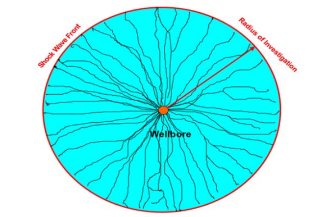
Figure 1 - Growing Clusters of Capillaries Behind a Shock Front


Eq. 2 is the same as the classic radius of investigation; Eq. 1 can be derived from simple calculus. However, Eq. 3 is a different concept to the conductive disc analogy (Earlougher 1977; Lee 1982; Matthews and Russell 1967) found in the literature. Instead of assuming that the reservoir is in communication with the entire reservoir the instant the well is placed on production, this proposed hypothesis presents the concept that until the shock front reaches a point in the reservoir, the pressure is constant. (Although it should be noted that if a reservoir has been in prior production, the pressure at ‘r’ may not be constant, but it will not be a function of the current location of the radius of investigation of the well that is being considered).
As a capillary network develops behind the shockwave boundary condition, small quantities of mass are rapidly transported along the opened capillary paths to redistribute the energy (pressure) and to satisfy the mass balance of each capillary. The transport mechanism is a damped inertial oscillation. The wave equation is derived using Darcy resistance, fluid capacitance and fluid inertia. The equation is written in terms of Darcy resistance for a capillary bundle. The resulting pressure wave moves rapidly up and down each opened capillary pathway from the wellbore to the capillary shockwave front and back again. The inertial term in the equation is non-zero and remains non-zero until some form of steady state (pseudo-, semi-, steady-) is reached. Once the reservoir reaches some form of steady state, the classic reservoir engineering equations for those flow regimes apply. However, in between the time that the radius of investigation encounters the first boundary and the start of some form of steady state, the physics and mathematics governing the pressure at any point within the radius of investigation is different than predicted by the classic transient flow equations.
Methods
The process of capillary growth during the early transient phase involves an elastic wave passing from the wellbore, out each active capillary, terminating at the primary capillary shockwave front (which marks the edge of the continuous bounded region), and back to the wellbore again. This mechanism allows the mass to redistribute in such a way that hydraulic power dissipation and heat generation are uniformly distributed throughout the field of flow. An equation can be written for flow or acoustic wave transport through a capillary. Darcy’s law as applied to porous media relates resistance-capacitance to porosity and utilizes bulk fluid velocity for the material balance on an element. In porous media the actual fluid velocity is some multiple of bulk velocity. It is the actual velocity that gives rise to inertial terms in the momentum equation.
Traditionally, these inertial terms have been eliminated as being small. Because we traditionally deal with bulk velocity in a critically damped porosity field (Hurst 1934), it is useful to understand the nozzle effect produced by the fluid being forced through the porous matrix. This acceleration term describes the characteristic velocity at which small amounts of energy and mass may be transported as a dynamic wave. If there were an effective means for producing an effective relative cross-section of flow area to total area, this could be calculated directly, while accounting for random porosity effects using a dynamic proportionality function, A, in the momentum equation. A simple case would involve the total cross-section of a single tube to the diameter of the tube bore. The ratio for that case is:

which may be considered to be the theoretical low end of the range of values for A. If this were the case, permeability would vary directly as porosity. However, field measurements indicate that the practical ranges for permeability – porosity correlations vary as an exponent or

where n ranges from 1.6 to 2.4 in individual field studies.
The diffusion equation used for field solutions has traditionally been derived by holding the inertial terms as being small (and set equal to zero) and of little consequence to the field solution (Hurst 1934). The concept of a critically damped field solution has long required that these small terms be discarded as insignificant. Nonetheless, these inertial terms are the principal means for energy transport within each capillary path in the reservoir and relate to the speed of communication within the reservoir.
Derivations of equations have traditionally been made using steady Poiseuille flow models for capillary tube bundles to derive Darcy’s law from simplified forms of the Navier-Stokes equations of fluid motion for Newtonian fluids (Hubbert 1956). The interaction of porosity and actual fluid velocity has been treated as a mass flux per unit area or bulk velocity process. However, when an acceleration term is included or a kinetic energy relationship is used, the process requires a correction to relate effective flow area to the actual area of the element of porous reservoir material.
The following derivation will add the dynamic term to the field diffusion model and derive a relationship for the inertial fluid acceleration through the formation. An inertial wave model will be used to describe mass redistribution in the radial network of capillaries. This supports the observation in well data that hydraulic power dissipation rapidly distributes itself throughout the region bounded by the capillary shockwave. The expansion velocity of the bounded region is much smaller than the velocity of mass redistribution within the region. Using this knowledge of wave or mass propagation in each capillary, a relationship between porosity, bulk velocity, and actual fluid velocity can be developed.
To avoid the complexities of phase interactions within the porous media, the derivation will be for a single-phase fluid. The compressibility of the mobile fluid phase will be modified by the compressibility of the matrix. Hence, the objective of this derivation is to establish a single-phase model that can be used to produce a relationship for compression wave passage and mass transport through porous media. An obvious future extension of this process would be to extend the solution process to multiple phases and the saturation for each phase.
Inertial Wave Model for a Capillary Bundle: Derivation
An element of porous reservoir media will be used to write a dynamic differential equation. The question arises as fluid flows through porous media as to how the restrictions imposed by the averaging of pores and throats at any cross-section in the reservoir will produce an acceleration effect upon the mass of fluid passing through the reservoir. The purpose of this exercise is to write a single dimensional equation for flow along a stream tube path.
The porous element will be defined around the concept of bulk flow, as is Darcy’s law. Since the impact of porosity on the acceleration term is not known, it will be necessary to introduce an acceleration coefficient A, which will allow the direct conversion of the actual velocity of the fluid element flowing through the reservoir element to be reconciled with the bulk velocity. The mass of the block is the fluid density of the transported phase times the volume of the cube times the porosity of the cube. The presence of another immobile phase in the block must be considered as a modification of porosity.
The method of solution is based upon writing a dynamic equation for fluid flowing through porous space in terms of Darcy resistance and bulk fluid velocity. Darcy’s law reconciles the shear stresses on the lateral faces of the fluid block to the normal face stresses applied as pressure to the faces of the block. The Darcy forces oppose the pressure gradient applied to the fluid block. The porosity fluid block and the porosity block will be written in terms of bulk velocity. The concept of sonic flow through a single capillary will also be used as the second relationship derivation.
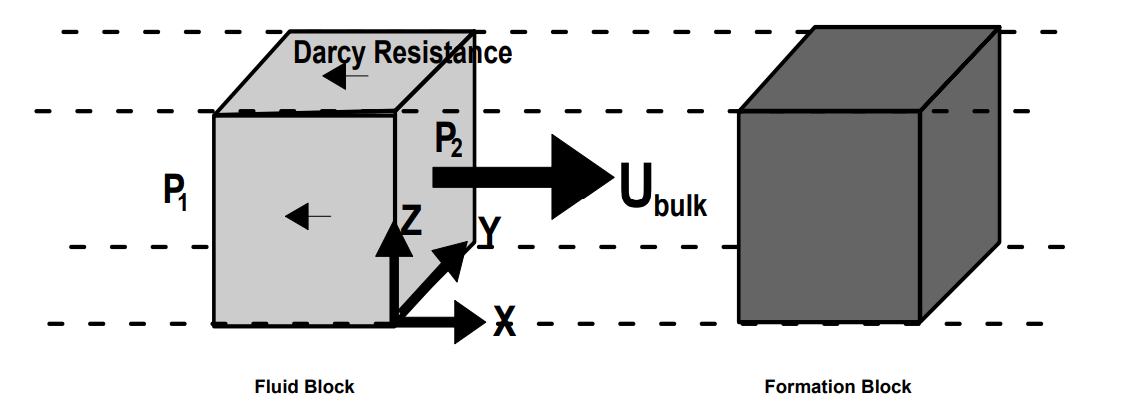
Figure 2 - Fluid Block Moving through Formation Block

The concept for this solution is based upon a fluid block passing through a block of formation. The formation occupies the volume (1-) *X*Y*Z and the fluid occupies the remainder of the volume * X*Y*Z. Visually, this is much like a body passing through another body. The resistance to flow of the fluid body through the formation can be represented as a shear stress on the lateral or streamline faces of the body, but through Darcy’s law resistance is relegated to an equivalent normal face stress on the fluid element (Hubbert 1956). The actual velocity of the fluid body is described by Darcy as the bulk flow through the porous medium. In order to correct for these differences, a differential equation will be written in terms of Darcy forces and the acceleration term will be corrected to actual velocity (and, hence, actual acceleration). The momentum equation is developed along a single dimension in the horizontal plane to the gravity force. This study will be limited to a unidimensional model. When equations are developed for the vertical dimension denoted by z then the gravity term will appear and can be dealt with through a transform of the energy equation. The static version of the energy equation was used by Hubbert (1956) to eliminate the gravity component and to restructure the equation in terms of potential flow. This eliminates the Bernoulli kinetic energy term and represents an assumption restriction on the diffusion model. This paper stops short of the introduction of flow potential.
First, the dynamic equation (Eq. 6a) is rearranged to eliminate common dimensional terms (Y and Z) and to make the derivative terms consistent, since P2 > P1:

Next, the momentum equation may be written in terms of Darcy’s law:

Defining A as the ratio of Uactual to Ubulk or:

Then Eq. 8 becomes:

Taking the derivative of the momentum equation with respect to x and rearranging terms:

The next step will be to rewrite the momentum equation in terms of pressure using the classic method of substitution of the Continuity equation:

To simplify the relationship, the assumption will be made that porosity and density changes with time and distance are essentially small relative to the two dominant terms. This is consistent with the concept of constant formation properties where /t =0 and small and constant compressibility of the fluid /x = 0 after Hubbert (1956).
This simplifies the relationship to Eq. 15:

Applying the chain rule and rearranging terms:

Compressibility is defined as the total system compressibility, Ct, so that the elasticity of the formation and connate fluids and their contribution to energy/mass transport are included.

Taking the derivative with respect to time:

Rearranging terms:

Substituting Eq.18 and Eq. 20 into the Momentum equation:

Rearranging terms we see a familiar equation for one-dimensional diffusive flow with an added term for inertia.

Note that the resulting Eq. 23 can be reduced to the classic diffusion equation for single dimensional flow (Hubbert 1956) if the second derivative of pressure with time is set to zero. This is not a new equation save for the inclusion of the time rate of change of momentum term. The equation can be rearranged into more familiar terms as Eq. 24 and 25.

A second check on the equation is to utilize dimensional analysis. This is facilitated by using hydraulic diffusivity and a mobility term based upon kinematic viscosity. Based on this relationship, it is evident that the inertial term becomes increasingly important as porosity, fluid density, and the velocity amplification ratio increase.
The Eigenvalue for the speed of the compression wave motion from Eq. 23 is:

The velocity of sound through the capillary is traditionally given by the relationship:

By using this relationship and equating the velocity of sound squared to the inertial wave:

Rearranging Eq. 28 to solve for A, cancelling terms and setting the result equal to Eq. 9:

The velocity of sound in the capillary has traditionally been assumed to be the transport mechanism. It is possible to consider some other limit to wave transport velocity as some fractional portion of the speed of sound. The terms would cancel resulting in the same relationship. This provides a mechanical flow equivalent to the Archie equation for the flow of electricity through porous media. This case assumed only one moving phase. A second phase present in the pore spaces will result in the modification of the compressibility and possibly result in a constant other than unity and a porosity exponent other than 2.
The general empirical equation form for the relationship can be written as:

Where the value of n is nominally 2.
The porosity-permeability relationship derives directly from the velocity model. Returning to the basic relationship of Eq. 30:

By comparing a change in the porosity for the same bulk velocity:

However, actual velocity is directly proportional to permeability (since permeability is an area) if viscosity, pressure gradient and bulk velocity are held constant:

Substituting the porosity and velocity relationships into Eq. 33 and Eq. 34 and equating as parallel members

As such, Eq. 36 may be written as a general relationship:

As such, Archie’s equation for electric current flow through porous media has a theoretical equivalent or analog for fluid flow through porous media.

Where n is approximately 2.
For an isotropic homogeneous porous medium the n value is 2 and provides the hydraulic equivalent of the Archie equation. However, in the real world of heterogeneous porous media, pore geometry and connective patterns produce different exponential values and coefficients for the permeability equation. This requires that permeability relationships be measured in situ by actual well tests.
Results: Diffusion Model Including Inertia
There are numerous factors besides the momentum effect of porosity that impact permeability. It is useful to understand the individual contributing factors that enter into the relationship and how they arise physically. In actual core measurements, there is generally a minimum porosity for which permeability is vanishingly small and a maximum range of porosities that can occur in nature. Further, porosity is a function of pore and pore throat geometry. Porosity may be impacted by particulates in the pores themselves that can result in statistical variations with actual fluid velocities. Eq. 26 describes the transport of small pressure waves in each capillary path as a function of the limiting velocity in the capillary. If the limiting Mach number is less than 1, the Mach numbers will cancel when the Eigenvalue terms are equated, leading to Eq. 39.

It should be noted that the last term of Eq. 39 is composed of individual terms that are finite, that is, non-zero. The definition of semi-steady state in terms of the second law of thermodynamics is that P/t will be a constant throughout the bounded region. This condition then leads to the result that the second derivative, 2 P/t2, is zero. However, by observation, it is repeatedly demonstrated that the pressure functions during transient behavior are straight-line functions of the log of time, connected by singular behavior changes or even small step pressure changes. None of these represents a zero second derivative, but in fact, lead to higher order derivatives for pressure. The second pressure derivative term must be considered in any model that deals with transient flow because porosity, density, fluid acceleration, compressibility, and the second derivative of pressure all have finite values in any formation that has permeability.
The compressibility value is a small number relative to the other numbers, but this is the term that gives rise to very high Eigenvalue velocities for pressure transport through the open capillaries. The transport velocity for redistributing small amounts of energy and mass in the system is several orders of magnitude larger than the propagation velocity of the bounding shockwave.
This is important to the understanding of the distribution of Joule-Thompson heat generation as a fluid flows through porous media. Because the system is dominated by the massive specific heat of the formation, Joule-Thompson heating is small and almost unmeasurable, but the pressure decay with time is easily and directly measurable with modern electronic pressure gauges. Because the boundary of the cone of influence expands very slowly, the distribution of power dissipation has ample time to equalize. It is the segregation of this energy in defined regions that provides the analyst information as to the gross features that the cone of influence has encountered.

In practical terms, when real values are placed into the velocity equations, it can be demonstrated that the bounding capillary shockwave moves at speeds of hundreds of feet per hour while the pressure waves moving behind the capillary shockwave are moving at hundreds of feet per second. Pressure (mass redistribution) is moving three orders of magnitude faster than the initiating capillary pressure boundary that confines the cone of influence. This suggests that the interior pressure distribution of the cone of influence is approaching semi-steady state conditions behind the slowly moving capillary shockwave boundary. Figure 3 shows the caricature overhead view of the capillary network, along with the differential equation that includes the inertial term (Eq. 39).
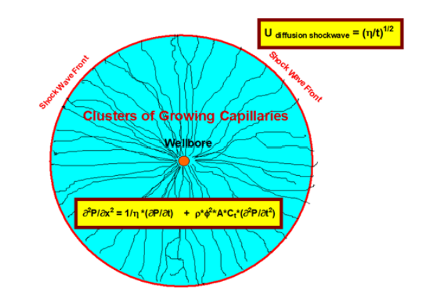
Figure 3 - Cone of Influence Structure and Waves that Bound and Redistribute Pressure
Results: Pressure Response in the Reservoir During Transient Flow and the Timing of the Arrival of the Secondary Shock Fronts Caused by the Primary Shock Front Striking Boundaries
The rapid communication along the radial structure of the cone of influence allows the effect of the slow-moving outer boundary to be decoupled from the redistribution of energy within the boundary. This leads to the recognition that pressure transients represent volume growth rather than pressure redistribution in a continuous field of flow. Pressure transients in porous media represent the interaction of a fast-moving inertial wave along open capillaries and a slow bounding shockwave. This radial redistribution is stabilized by the substantial mass of fluid moving radially inward to the wellbore. Once flow is established along a radial pattern, the formation remembers this pattern in two ways. The first is capillary memory and the second is radial inertial inflow. The cone of influence bounded by the shock front coincident with the radius of investigation is best described as a massive fluid flywheel. The mass of a 100 BCF reservoir is the equivalent of five half million-ton supertankers all headed to the same point.
If both the concept of the fast-moving inertial wave and the slow-moving shock wave (radius of investigation) are included in the derivation of the radial flow equations, a different picture of transient flow emerges. Instead of a smooth relaxation curve from the edge of the reservoir to the well, (Earlougher 1977; Lee 1982), the pressure responses both at the well and in the reservoir have distinct log-linear (pressure vs. log time) features which are piecewise discontinuous. These discontinuities are caused by the radius of investigation striking a boundary.
As mentioned before, there is absolutely nothing wrong with the classic equation for transient flow in a reservoir in infinite acting radial flow, as long as the point of observation is within the radius of investigation. However, once boundaries are encountered, but before the system enters some form of steady state, an increasingly nested series of equations is required.
The secondary shock fronts caused by the primary shock wave striking a boundary gain volume at a rate that is equivalent to the volume that the primary shock front is no longer gaining (Goldsberry 1998). They travel out from the well, positioned at a distance R as a function of time (note that there are multiple secondary shock fronts, each nesting inside the other like a matryoshka doll). Eq. 41 presents the equation used to solve for the position of the secondary shocks.

The velocities of the secondary shock waves are simply the derivative of the position:

As more and more boundaries are encountered, the system of conditional equations used to describe pressure across the reservoir can be created based on the time from startup that the boundaries are encountered:

For the producing well, the skin term must also be applied in Eq. 43 (Lee, 1982, Eq 1.11), by substituting the wellbore radius rw for r and subtracting two times the dimensionless skin (s) from the Ei term, as shown in Equation 43b. However, the skin does not apply outside of the damaged/stimulated region around the well, as has been amply described by Lee; thus, will not be considered further for the sake of brevity.

Equations 43 and 44 form the basic equations for pre-boundary transient flow. Each boundary causes an additional term/ratio to be added to both the P(r,t) function and the conditional statement list. For the following equations and conditions (Eq. 45-51), a subscript number will be used to indicate which boundary is the reference. Boundaries are struck in sequence, so subscript ‘1’ refers to the first boundary and the first secondary shock wave. The infinite acting radial flow portion will be subscripted as ‘0’ (referred to as the mid-time slope elsewhere) and reference the primary shock front (Ri). Note that all Mn slopes are observed at the producing well.
After the first boundary is encountered, Eq. 43 will become:


After the second boundary is encountered and continuing until the n’th boundary, there are increasing numbers of moving boundary conditions (shocks) in the system. This makes the mathematics a bit tedious. In lieu of a lengthy derivation, only the final equation and conditional statements will be presented.
Equation 48 is the general solution for n > 1 boundaries. Eq. 50 describes the scalar correction that needs to be applied to account for the discontinuities at the shocks.
Please note that a substitution of -Ei(-x) = -ln(1.781 x) has been made, in order to simplify the math.

Where ????ሺ????, ????ሻ|ିଵ is the pressure value of the shock region before the new shock arrives and ????ሺ????, ????ሻ| is the value determined from the first two terms of Eq. 48. ∆???????????????? is the capillary threshold pressure change induced by the n’th shock front. It is usually less than 1 psi and can be neglected for moderate and low permeability rock. It should be noted that Eq. 50 should be evaluated at the time t corresponding to the arrival of shock n (tn). The conditional statement for n > 1 boundaries is:

The following case history will demonstrate how these equations match real data.
Field Data Supporting the Proposed Solution to the Diffusivity Equation Including the Inertial Term
The following data were acquired during a test in the Gulf of Mexico. In order to prove continuity between the two wells, one well (P1) was produced on a constant choke for 18 days, while the second well (O1) was shut in/observing the response in order to establish communication with the producer. The observation well was equipped with a downhole gauge set 300 feet above the completion. A downhole gauge was also run in the producing well to the top of the completion prior to the final shut-in at the end of the test to record the build-up. The wells were on strike. This difference in gauge depth will cause a difference of about 15 psi between the two measurements. The pressure data has not been altered or smoothed in any way, hence the noise in the pressure response.
The wells were 2000 feet apart laterally at reservoir depth. P1 produced single-phase gas at 17 MMscf/D with almost no variation and no flow interruptions or choke change during the test. O1 was shut-in the entire time P1 was producing. Table 1 lists the parameters used for the determination of the permeability and hydraulic diffusivity.
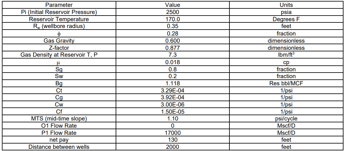
Table 1 - Case Study Well Test Input Parameters
This leads to a base build-up permeability of 360 md, which becomes 224 md after correcting for elasto-plasticity of the formation. Using permeability of 224 md and the appropriate input parameters above, the hydraulic diffusivity is 35645 ft2/hour.
Two boundaries were observed in the build-up in the Producing well (P1) at 1.8 and 3.7 hours delta time. These are shown in Figure 4. Note that the graph is plotted on an inverse scale, with the pressure declining on the left y-axis, in order to compare it with the drawdown in the observation well (O1).
Figure 4 - P1 Build-up Plotted on Inverse Scale (Pressure Increasing Down)
Based on the hydraulic diffusivity and the other input parameters in Table 1, the distance to the limits may be calculated using Eq. 2 and the timing of the arrival at the interference well may be determined using Eq. 2, rearranged to solve for time, setting Ri to 2000 feet. Next, Eq. 49 can be rearranged to solve for time and the arrival time of the secondary shocks may be calculated. Table 2 presents the boundary contact times and the Mn slope values from the build-up.

Table 2 - Boundary Times and Slopes
Table 3 presents the calculated boundary distances from P1 and times of arrival of the primary and secondary shock fronts at O1.

Table 3 - Timing of Events in Producer and Observer
Figure 5 shows the actual field data from the observation well, showing the arrival of the primary and first two secondary shocks, with the arrival times annotated on the graph. Note that the predicted arrival times of all of the shock fronts coincide with the actual arrival times. The semi-log scale of time is the ‘old school’ format, with five divisions for the first three units of a log cycle and two divisions for the units from four to ten. The major tick marks are below the x-axis.
Figure 5 - Arrival Times of Shock Fronts at the Observation Well (O1)
The arrival of the primary shock (the radius of investigation) is preceded by nothing but gauge noise, not a smoothly decaying relaxation curve. The ‘railroad tracking’/double line seen in the plot is caused by a lack of resolution in the temperature compensation of the quartz gauge. However, the shift in slope marking the arrival of the shock fronts are still obvious. This indicates that the results of the solution to the diffusivity equation derived here using both initiating capillary pressure and inertia within the bounded region (along with strict adherence to the second law of thermodynamics) are at least reasonable.
If the build-up in the producer on an inverted scale is plotted against the drawdown with the reference time adjusted to match the arrival of the primary shock front, every single bobble in the pressure data from the build-up in P1matches a similar response in the drawdown in O1, indicating that these responses are caused by the reservoir geometry. This overlay is shown in Figure 6.
Figure 6 - Overlay of the Inverse PBU in P1 and the Drawdown in O1
Finally, in Figures 7 and 8, the O1’s downhole gauge data is digitized, offset to completion depth (+15 psi), then compared to the predicted pressure profile generated from Eq. 48 and Eq. 50, with conditional statement 51. Both a Cartesian and a Semi-log plot are presented.
Figure 7 - Comparison of O1 Actual BHPs and Predicted BHPs (Cartesian)
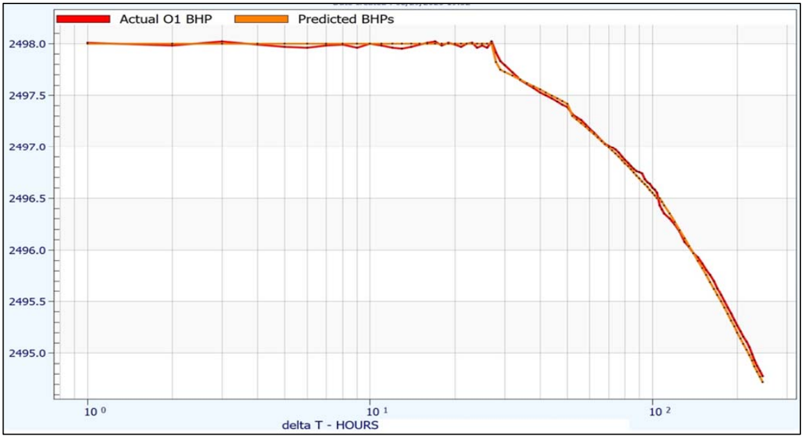
Figure 8 - Comparison of O1 Actual BHPs and Predicted BHPs (Semi-log)
Thus, Equations 43-51 not only accurately predict the arrival time of the primary and secondary shock fronts, they also predict the pressure response at the observation well location. Furthermore, it should be noted that there are distinct shifts in the slope of the pressure response. This segmented response in both wells and the coincidence of events should be the final nail in the coffin for the idea that transient flow should be governed by a simple relaxation curve. Figure 9 demonstrates a more appropriate visualization of the reservoir in post-boundary radial flow.
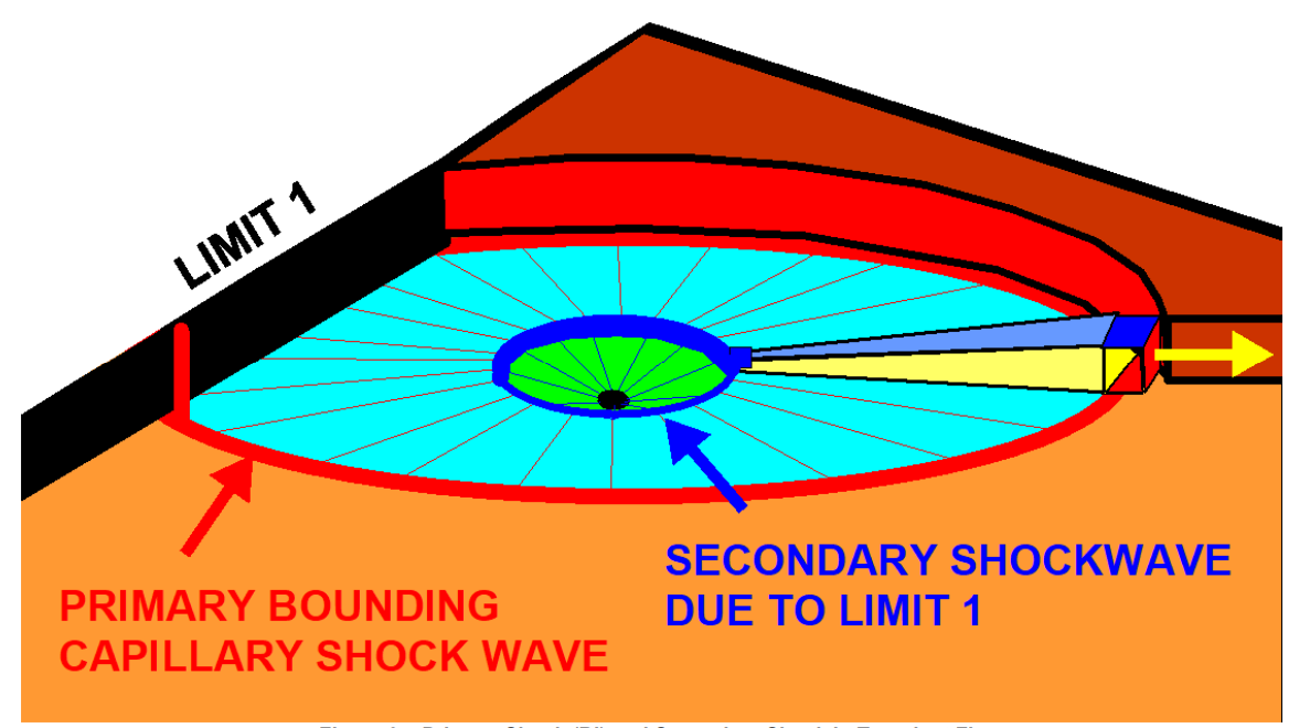
Figure 9 - Primary Shock (Ri) and Secondary Shock in Transient Flow
Conclusions
In order to understand and properly model the pressure response at the well and in the reservoir during transient flow, both inertia and capillary entry/threshold pressure must be included in the solution to the diffusivity equation.
Before encountering any boundaries, the radius of investigation is not simply an inflection point of a mathematical construction of a relaxation curve, it represents a physical shock front that separates active reservoir volume (dominated by the producing well) from inactive reservoir volume. During pre-boundary/infinite acting radial flow, reservoir volume growth is linear with time (i.e. if 1 million barrels were observed in 3 hours, 2 million barrels will be observed in 6 hours).
The inclusion of inertia in the solution to the diffusivity equation is required to impose a second law thermodynamic constraint on the active system. The inclusion of capillary threshold pressure at each rupturing pore throat provides a moving boundary condition. It also allows for a capillary structure with finite wall strengths. Through continuity, the energy equation (first law of thermodynamics) and the inertial wave equations derived in the paper (second law of thermodynamics’ constraint), a more rigorous physical and mathematical model has been developed to explain and predict the behavior of transient flow at any point in the reservoir.
Afterword
With this derivation and discussion, the majority of the concepts that make up “WaveX Theory” have now been published (Goldsberry 1998, 2000; Fair and Goldsberry 2012). The focus of this paper was the importance of the inertial term in the diffusivity equation. Papers published in 1998 and 2012 addressed the importance of capillary entry/threshold pressure. The point of this work has been to try to find a physical explanation for the segmented, log-linear (with time) behavior observed in real field pressure data from build-ups and drawdowns, as well as to be able to predict the arrival of secondary shock events and, in general, the pressure response in a reservoir between the time the first boundary is contacted until the well/reservoir enters some form of steady state (pseudo-steady state, steady state, etc.).
As this paper is mostly theoretical, the authors plan future publications discussing the practical application of this and the previously published material. The following is a list of topics that the authors intend to address in the future (although additional contributions and suggestions from the industry would be appreciated):
1) The end of the effective drainage area in tight/unconventional reservoir
2) Well test planning with shock fronts
3) The transition period between the end of transient flow and the beginning of some form of steady state flow
4) The recognition of boundary contact types (fault, strat, water contact, etc.)